1. Introduction
2. Materials and Methods
2.1 Materials
2.2 Methods
3. Results and Discussion
3.1 Principal component analysis
3.2 Model evaluation and comparison
3.3 Feature importance
3.4 Classification of unknown classes
4. Limitations and future studies
5. Conclusions
1. Introduction
Criminals have been able to utilize advanced technology and various methods over the last ten years to achieve organized crimes. As advancements in science and technology progress, criminals are becoming increasingly adept at incorporating emerging scientific technologies into their illicit activities and motivations for engaging in criminal behavior. In the field of forensic document examination, experts confront a growing challenge as intricate criminal cases present complexities in differentiating between genuine and forged documents, identifying and authenticating paper documents.
Through actions such as tax evasion, bank fraud, counterfeiting and other financial crimes, increased criminal activity has an economic impact. When this situation arises, the documents to be examined must be thoroughly investigated by a scientist using non-destructive methods in order to preserve their evidential value. In a forensic laboratory, the most common requests for the analysis of paper relate to the date and place of its manufacture.1) Typically, paper discrimination has involved evaluating a range of physical and optical characteristics, including tensile strength, thickness, basis weight, ash content, color, and fluorescence.2) However, these methods have difficulty in matching two sheets of paper correctly and reliably3) and require fairly large sample sizes. As advances in science and technology have progressed, a variety of methods have been used to analyse the paper. Various methods have been proposed to carry out investigations, including X-ray diffraction,4,5,6,7) elemental analysis,8,9) infrared spectroscopy,10,11,12) Raman spectroscopy,13) image analysis14) and pyrolysis gas chromatography.15)
Machine learning technologies, including support vector machines, artificial neural networks, random forests, and others, are being applied across various fields. Recently, these approaches have been regarded as valuable tools in the forensic field to address time-consuming tasks. Spectral data, such as UV-Vis, infrared, and Raman spectra, have proven suitable for building machine learning models and have been used to examine paper materials.16,17,18,19,20) Combining machine learning with various analytical data has shown significant promise for paper examination. For instance, Lee et al.21) performed classification tasks on seven types of document paper, achieving an accuracy of 97.6%. Their method integrates texture features extracted from visible light transmission images and infrared transmission images using the gray-level co-occurrence matrix approach. Additionally, a convolutional neural network extracts another set of features from the same images. This dual-feature extraction process significantly enhances the accuracy of model and reliability.
Boosting is a powerful ensemble learning technique that combines the predictions of several base estimators to improve robustness and accuracy.22) Unlike bagging methods23) that build multiple independent models, boosting algorithms train models sequentially, with each new model correcting the errors of its predecessor. Three boosting algorithms are adaptive boost (Adaboost), gradient boosting machine (GBM), and extreme gradient boost (XGBoost). In this study, 2D lab formation data were used to develop models for forensic paper examination. The dataset includes intensity, step, and angle measurements derived from lookthrough images of paper samples.
2. Materials and Methods
2.1 Materials
The details of the copy paper utilized in this study are presented in Table 1. 2D Lab Formation Sensor (Techpap, France) was employed to analyze both sides (front and back) of a piece of copy paper. The data collection process was repeated to acquire a total of 50 samples. The data that was scanned from one side of the paper was displayed as a 50 × 20 matrix, as step and angle values were calculated based on the top 10 intensity in the measurement. Finally, a classification model was constructed using the 500 sample dataset (50 samples of 10 categories each).
Table 1.
Information regarding the copy paper produced by various manufacturers
| No. | Sample | Country | Basis weight, g/m2 |
| 1 | CP1 | Korea | 80 |
| 2 | CP2 | Korea | 75 |
| 3 | CP3 | Japan | 75 |
| 4 | CP4 | Japan | 90 |
| 5 | CP5 | Japan | 85 |
| 6 | CP6 | China | 70 |
| 7 | CP7 | Indonesia | 80 |
| 8 | CP8 | Thai | 80 |
| 9 | CP9 | USA | 75 |
| 10 | CP10 | Brazil | 80 |
2.2 Methods
2.2.1 Angle and step data
The paper samples were positioned on the sensing area of the 2D-F sensor in the machine direction, and an image of the transmitted light was captured. The step and angle values were determined using the Fast Fourier Transform (FFT) algorithm of the Techpap image analysis software (EPAIR). A step refers to the distance in millimeters between periodic marks, while an angle denotes the orientation of the linear periodic mark.
2.2.2 Data preprocessing
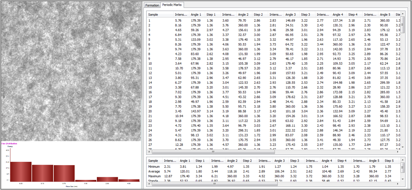
Fig. 1 shows the light-transmitted image and the intensity, angle, and step data from the Techpap image analysis software during the analysis using a 2D F sensor. To ensure that the top 10 angles and step data were sufficiently variable according to intensity, preprocessing was performed by sorting the data so that larger steps were aligned. Additionally, the intensity variable was removed from the dataset. For the angles, since values like 75 degrees and 105 degrees are essentially the same, they were pre-processed by taking the absolute value of the sine function. Specifically, the dataset was sorted in decreasing order, and the top 10 values were transformed using the absolute value of the sine function. The processed data then combined these transformed angles with the next set of step data.
2.2.3 Data splitting
The datasets were divided into training and testing sets with a ratio of 7:3 to facilitate the modelling and evaluation of the classification models. To ensure that the split ratio was maintained for each class, stratified random sampling was employed during the partitioning process.
2.2.4 Principal component analysis
Principal Component Analysis (PCA) was conducted to identify meaningful patterns or structures within the dataset. The dataset was transformed into a new orthogonal coordinate system, consisting of five principal components (PCs). Subsequently, the transformed data points were visualized in a two-dimensional (2D) space.
2.2.5 AdaBoost
AdaBoost is an effective classification algorithm that aims to maximize the minimum margin of a training sample.22) In this study, the SAMME24) algorithm was applied to the angle and step dataset for multi-class classification. This boosting algorithm was employed to improve classification performance by iteratively adjusting the weights of incorrectly classified instances and combining multiple weak classifiers to form a strong classifier. Classification trees were utilized as the base classifiers.25) To further optimize the model, a grid search was conducted by varying the maximum depth (‘maxdepth’) and the number of iterations (‘mfinal’). The parameters explored ranged from 3 to 5 for ‘maxdepth’ and 10 to 300 for ‘mfinal’.
2.2.6 Gradient Boosting Machine
Gradient Boosting Machine (GBM) utilizes gradient descent to optimize the loss function, which quantifies the discrepancy between the actual and predicted values.26) During each iteration, GBM calculates the gradient of the loss function with respect to the predictions made by the ensemble model. This gradient information is then used to update the model by incorporating a new weak learner, typically a decision tree, that aims to reduce the residual errors. Key hyperparameters in GBM include the distribution type, the number of trees (‘n_trees’), the maximum depth of the trees (‘maxdepth’), the learning rate (‘lr’), and the minimum number of observations in a node (‘n_minobsinnode’). For the multi-class classification task, the ‘multinomial’ distribution was chosen. A grid search was employed to find optimal values for the ‘maxdepth’ and ‘n_trees’, with ‘maxdepth’ ranging from 3 to 5 and ‘n_trees’ ranging from 10 to 300. The learning rate and the minimum number of observations in a node were kept constant at 0.1 and 10, respectively.
2.2.7 XGBoost
The eXtreme Gradient Boosting (XGBoost) algorithm enhances prediction performance by aggregating the predictions of multiple weak learners to form a robust model.27) XGBoost differs from traditional Gradient Boosting Machines (GBM) through its implementation of second-order gradient optimization and parallel processing, leading to more precise and efficient model training compared to the first-order gradient optimization used in GBM. For multi-class classification tasks, the number of classes was set to 10. The learning rate (eta) was set to 0.1, and the maximum depth of the trees ranged from 3 to 5. The model was trained for 300 rounds using these parameters.
In the context of modelling with the XGBoost algorithm, Feature importance was assessed using the Mean Decrease Impurity (MDI) method.28) This approach calculates the importance of each variable based on the average reduction in Gini impurity, thereby identifying which variables contribute most significantly to the decision making of model.
2.2.8 Model evaluation
Assessing the accuracy of classifying observations into positive and negative categories is critical in classification tasks. True positives (TP) denote correctly classified observations belonging to the positive class, whereas true negatives (TN) refer to correctly classified observations belonging to the negative class. Conversely, false negatives (FN) occur when positive observations are incorrectly classified as negative, and false positives (FP) occur when negative observations are incorrectly classified as positive.
Several performance metrics derived from these values are essential for evaluating the classifier’s ability to detect the target class. Commonly used indicators include specificity, sensitivity, and accuracy.29,30) The formulas for calculating these metrics are as follows: accuracy is calculated as (TP + TN) / (TP + TN + FP + FN), sensitivity is calculated as TP / (TP + FN), and specificity is calculated as TN / (TN + FP).
The R statistical software (R Core Team, version 4.4.1, Auckland, New Zealand) was primarily utilized for all data processing and classification procedures in this study.
3. Results and Discussion
3.1 Principal component analysis
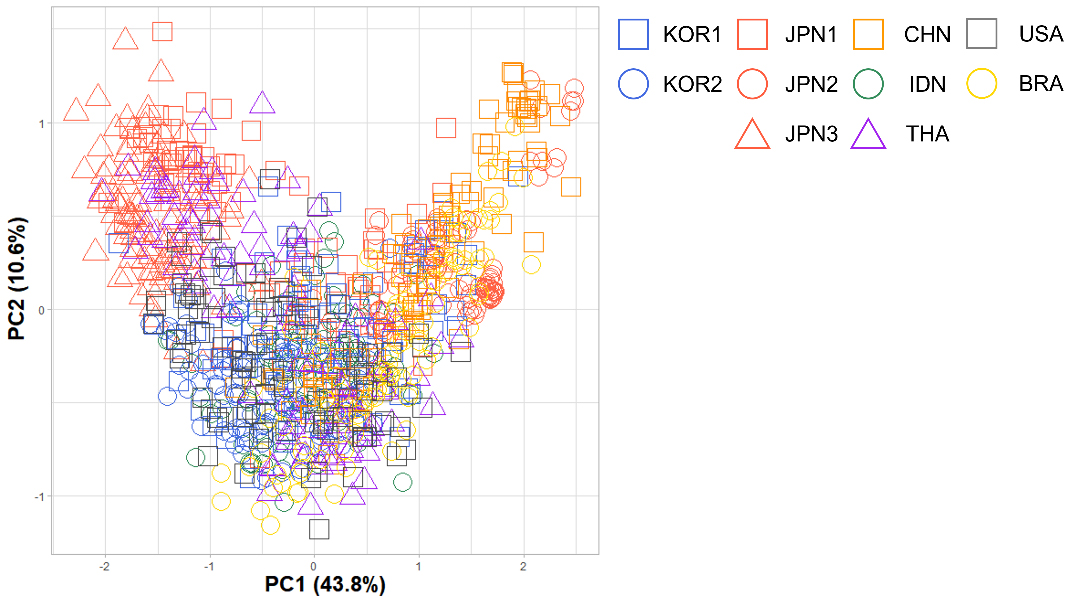
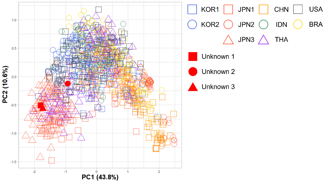
Fig. 2 shows the PCA score plot for the first two principal components (PCs) derived from the angle and step data. The dataset was pre-processed by sorting the data to align larger angles and steps, and the intensity variable was excluded due to its variability. Angles were further pre-processed by applying the absolute value of the sine function. In the PCA score plot, data points are observed to either cluster together, as seen with JPN3, or separate into distinct clusters, such as the THA samples. These clustering patterns are attributed to the types of paper machines used. For instance, in a single-wire system like the Fourdrinier machine, the paper exhibits consistent marks on both the top and bottom sides of each sheet. In contrast, a twin-wire system, such as those used in hybrid and gap former machines, can produce different marks on the top and bottom sides of the paper.
3.2 Model evaluation and comparison
The classification performance of AdaBoost, GBM and XGBoost is compared in Table 2. The observed differences in classification performance can be attributed to the distinct mechanisms underlying each algorithm. AdaBoost improves model performance by sequentially adjusting the weights of incorrectly classified instances and combining multiple weak classifiers, typically decision trees, to form a robust ensemble.31) However, its performance may be limited by its sensitivity to noisy data and its reliance on a series of weak models.
Gradient Boosting Machine (GBM) builds upon the concept of AdaBoost but utilizes gradient descent to minimize the loss function more effectively. GBM constructs trees in a stage-wise fashion, with each tree correcting the errors of its predecessors, which often results in improved accuracy compared to AdaBoost.32) Nevertheless, GBM may still be subject to overfitting if not properly regularized.
XGBoost extends the principles of GBM by incorporating advanced techniques such as second-order gradient optimization and parallel processing, which enhance both the precision and efficiency of model training.27) Its ability to handle complex patterns and interactions, coupled with regularization to prevent overfitting, contributes to its superior performance in achieving the highest accuracy among the three models evaluated.
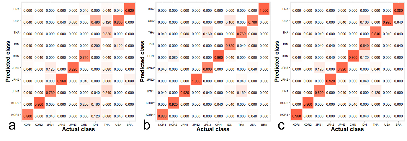
Sensitivity (Sen.) measures the proportion of true positives correctly identified by the model, reflecting its ability to detect positive instances. Specificity (Spe.) assesses the proportion of true negatives correctly identified, indicating the model’s effectiveness in recognizing negative instances. As shown in Table 2, the sensitivity for IDN and THA in each model was notably low. This may be attributed to the characteristics of the paper machines, as discussed in the PCA results (Fig. 2). The different marks on the top and bottom sides of the paper increase class discrepancies, complicating the models’ decision-making processes.
Table 2.
Comparison of model performance
Fig. 3 shows the confusion matrices for the classification results of each model, providing a detailed breakdown of true positives, true negatives, false positives, and false negatives for each model.
3.3 Feature importance
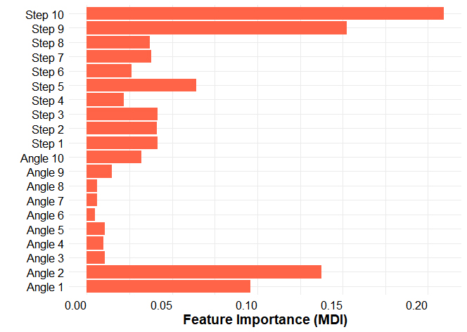
Fig. 4 shows the feature importance of XGBoost based on Mean Decrease Impurity (MDI). The variables depicted in Fig. 4 were presented after preprocessing, with the values shown being independent of the intensity variable. In this context, higher values indicate that a variable is ranked closer to the 1st position, while lower values suggest a ranking closer to the 10th position.
For angle data, angles of 180 or 360 degrees yielded the lowest values after applying the absolute sine function, which resulted in these values being ranked in the 10th position. These angles are considered to have low importance, as depicted in Fig. 4. This is because they correspond to the cross direction (CD) in the papermaking process, where weave marks on the forming fabric are prevalent across all products. In contrast, angles near 90 or 270 degrees, which yielded the highest values after applying the absolute sine function, are regarded as highly important. These angles correspond to the machine direction (MD) and can be attributed to both weave marks and drainage marks. While weave marks may be consistent across products, drainage marks are likely to exhibit unique characteristics influenced by factors such as machine speed and wet-end processes. Thus, it is inferred that these variables are of greater importance.
Similarly, for step data, relatively large step values that arise from weave marks are expected to be ranked highest. Therefore, the step data ranked 9th and 10th in importance are likely to reflect gaps originating from drainage marks rather than from weave marks. This is because drainage marks exhibit unique characteristics depending on the manufacturer, making them potentially valuable features for forensic examination.
3.4 Classification of unknown classes
Non-specified samples, labeled as Unknown 1 to 3, were analyzed using the XGBoost classifier for forensic document examination. The classifier predicted these samples as belonging to JPN2, THA, and JPN2, respectively. Fig. 5 illustrates the PCA score plot, depicting the first two principal components derived from the angle and step data, with the unknown classes indicated.
4. Limitations and future studies
This study focused on the classification of document paper for forensic purposes using a 2D Lab Formation sensor with boosting algorithms. The performance of models trained with data from both the top and bottom sides of the paper exhibited unavoidable bias. Additionally, the models were trained using angle and step data from specific lots. As the forming fabric is a consumable product replaced every one to two months, the training datasets need to be updated frequently to maintain robust models. Notably, advancements in forming fabrics aimed at enhancing retention properties, drainability, and formation further necessitate a comprehensive and large dataset to accurately detect manufacturer and manufacture date. For forensic applications, deep learning-based document detection models that encompass both manufacturer classification and document dating would be more appropriate. Future research will focus on developing deep learning models for document dating.
5. Conclusions
1. The angle and step data from the 2D Lab Formation Sensor were introduced to investigate forged documents. For machine learning approaches, these data were preprocessed using a sorting method and angle transformation.
2. The PCA score plot revealed that some data classes tended to separate into binary clusters depending on whether the data were obtained from the top or bottom side of the paper sheets. This characteristic is attributed to the paper machine, whether it uses single wire or twin wire systems.
3. Boosting algorithms such as AdaBoost, GBM, and XGBoost were tested with the angle and step data. XGBoost outperformed the others, achieving an accuracy of 0.880.
4. MDI-based feature importance was measured from the XGBoost model, identifying the angle and step data derived from drainage marks as high-importance variables.


