The Feasibility of Cross Hedging Wood Pulp with CME Lumber Futures

Min Su Kim; Seon-Woong Kim; Byung-Sam Yoon

doi:10.7584/JKTAPPI.2019.10.51.5.38

Preview

Journal of Korea TAPPI. 30 October 2019. 38-44
https://doi.org/10.7584/JKTAPPI.2019.10.51.5.38

The Feasibility of Cross Hedging Wood Pulp with CME Lumber Futures

Min Su Kim¹

Seon-Woong Kim¹

Byung-Sam Yoon¹^†

¹Department of Agricultural Economics, Chungbuk National University, Chungbuk, 28644

^†Corresponding author: E-Mail: bsyoon@cbnu.ac.kr

ABSTRACT

The main objective of the study is to determine whether the CME (Chicago Mercantile Exchange) random length lumber futures can be used as a cross hedging vehicle for the wood pulp (LBKP and NBKP). In order for the cross hedging to be feasible, there should be a strong positive relationship between the cash price and the futures price. This study conducted rigorous statistical analyses such as cointegration test and Granger causality test to examine the price relationship between CME lumber futures and wood pulp. The empirical analyses suggest that CME random length lumber futures can not be used as a potential cross hedging vehicle for wood pulp.

Keywords

Cross hedging

wood pulp

LBKP

NBKP

CME random length lumber futures

hedge ratio

hedging effectiveness

MAIN

1. Introduction

Wood pulp is the main component in the papermaking process. The pulp and paper industry in Korea depends heavily on imported pulp for the manufacturing of various paper products. In 2017, the volume of pulp consumed was 2,738,179 metric tons, of which 82.8% was imported and 86.3% was chemical pulp.

It is well known that the wood pulp market is highly volatile. In fact, it has become increasingly unstable. Wood pulp costs directly impact paper prices, and ultimately impact the profitability of the pulp and paper industry. An increase in wood pulp price leads to decreasing profits for paper companies that buy wood pulp as raw material. Thus, paper companies face the risk of rising pulp prices. On the other hand, a decrease in wood pulp price leads to decreasing profits for pulp companies that sell wood pulp as the final product. Thus, pulp companies face the risk of falling pulp prices. Effective price risk management is critical for the pulp and paper industry.

When it comes to hedging price risk in commodities, the most commonly used derivative instruments are futures contracts. While paper companies that use wood pulp can hedge against increasing wood pulp prices through buying wood pulp futures contracts, pulp companies that produce wood pulp can hedge against decreasing wood pulp prices by selling wood pulp futures contracts. Unfortunately, there is no viable futures market for wood pulp, consequently pulp and paper companies cannot directly hedge their price risks in the wood pulp futures market.^[1] However, there is a wood-related futures contract traded in the Chicago Mercantile Exchange (CME), CME random length lumber futures. Thus, pulp and paper companies may have the opportunity to cross hedge wood pulp prices with CME random length lumber futures contract.^[2]

This paper aims to determine the feasibility of cross hedging wood pulp with CME random length lumber futures. In order for the CME lumber futures to be used as a potential cross hedging vehicle for wood pulp, there should be close price correlations between wood pulp and CME lumber futures. In other words, they should have similar price movements.

2. Materials and Methods

2.1 Data

Cash prices for wood pulp are obtained from the Korean Statistical Information Service (KOSIS). The cash prices are monthly average prices for LBKP (laubholz bleached kraft pulp) and NBKP (nadelholz bleached kraft pulp) respectively. While LBKP is the hardwood kraft pulp made from trees with leaves, NBKP is the softwood kraft pulp made from trees with needles. The prices are based on cost, insurance and freight (CIF) values for imported wood pulp and quoted in dollars per ton ($/t).

Futures prices are the daily settlement prices of the CME random length lumber futures (RLLF).^[3] The futures prices are obtained from a computer database compiled by Reuters. Since cash prices are monthly average prices, monthly averages of the nearby futures price series are used for futures prices. When constructing nearby futures price series by continuously connecting the nearby futures prices, we roll over to the next nearest contract on the last trading day (LTD) of CME RLLF.

The sample period extends from January 2003 through June 2019, resulting in 198 observations. The natural logarithms of the prices multiplied by 100 are used, since both cash and futures returns are conventionally assumed to follow log-normal distributions.

2.2 Methods and procedures^[4]

2.2.1 Unit root test

A unit root test is used to test whether a time series variable is non-stationary and possesses a unit root. The presence of a unit root is tested by employing the ADF (augmented Dickey-Fuller) test using Eq. 1. The null hypothesis is that the time series has a unit root and is non-stationary.

[1]

Δ y_{t} = α + β t + γ y_{t - 1} + \sum_{i = 1}^{p - 1} δ_{i} Δ y_{t - 1} + ε_{t}

where yt=(S_t, F_t), S_t is the cash price for LBKP and NBKP respectively, and F_t is the CME RLLF price. t represents a time trend, and ∆ represents a differencing operator such that ∆y_t=y_t-y_t-1.

2.2.2 Cointegration test

Given that two time series variables are integrated of order one, or I(1), respectively, a cointegration test is used to test whether they share a common stochastic trend. To determine the cointegration relationship or long-run equilibrium relationship between wood pulp and CME lumber futures prices, the Johansen’s multivariate cointegration procedure is used. The Johansen approach proceeds with the general form of a pth order vector autoregressive (VAR) model.

[2]

y_{t} = δ + Φ_{1} y_{t - 1} + \dots + Φ_{p} y_{t - p} + ε_{t}

where y_t is a vector consisting of the cash price (S_t) for LBKP and NBKP, respectively, and the CME RLLF price (F_t). δ is a vector of constants. ε_t is a vector of error terms satisfying the multivariate normal white noise process with mean 0 and finite covariance matrix Σ.

The VAR(p) above can be reparameterized into a vector error correction model (VECM) of the following form.

[3]

Δ y_{t} = δ + Π y_{t - 1} + Γ_{1} Δ y_{t - 1} + \dots + Γ_{p - 1} Δ y_{t - (p - 1)} + ε_{t}

Where $Π = (\sum_{i = 1}^{p} Φ_{i} - I), and Γ_{i} = - \sum_{j = i + 1}^{p} Φ_{j}$

Johansen³⁾ shows that the coefficient matrix Π contains essential information about the cointegrating or equilibrium relationship between the variables. Specifically, the rank of Π matrix is equal to the number of independent cointegrating vectors. Based on the mathematical properties that the rank of a matrix is equal to the number of its characteristic roots (eigenvalues) that differ from zero, the test for cointegration between the variables can be conducted using the following maximum eigenvalue test (λ_max) statistics.

[4]

λ_{max} (r, r + 1) = - T ln (1 - {\hat{λ}}_{r + 1})

The maximum eigenvalue statistic (λ_max) tests the null hypothesis that the number of cointegrating vectors is r against an alternative hypothesis of r+1 cointegrating vectors. In this study, y_t=(S_t,F_t)' and so the number of variables is 2. The hypothesis of cointegration between S_t and F_t is equivalent to the hypothesis that r=1. If r=0, then the two variables are not cointegrated.

2.2.3 Vector autoregressive (VAR) model and granger causality

The temporal relationship between the variables can be studied simultaneously by estimating the vector autoregressive (VAR) model. In order to determine the price discovery and lead-lag relationship between the wood pulp and CME RLLF prices, the following VAR model is estimated.

[5]

Δ S_{t} = α_{s} + \sum_{i = 1}^{m} β_{s i} Δ S_{t - i} + \sum_{j = 1}^{m} γ_{s j} Δ F_{t - j} + ε_{s t}

[6]

Δ F_{t} = α_{f} + \sum_{i = 1}^{m} β_{f i} Δ S_{t - 1} + \sum_{j = 1}^{m} γ_{f j} Δ F_{t - j} + ε_{f t}

where ∆ denotes the differencing operator. ∆S_t is the change in cash price for LBKP and NBKP respectively, and ΔF_t is the change in CME RLLF price. ε_st and ε_ft denote white noise errors with zero mean and constant variance.

In Eqs. 5-6, Granger causality tests are associated with tests on the significance of the coefficients γ_sj and the β_fi conditional on the optimal lag length m.^[5] In Eq. 5, if all the coefficients of γ_sj are equal to zero, implying that past changes of F_t have no explanatory power for the current change of S_t, then F_t does not Granger cause S_t. This is formally tested using the null hypothesis H₀ : γ_s₁ = γ_s₂ = ⋯ = γ_fm = 0 and concluded that F_t Granger causes S_t if the hypothesis is rejected.

Similarly, in Eq. 6, if all the coefficients of β_fi are equal to zero, implying that past changes of S_t have no explanatory power for the current change of F_t, then S_t does not Granger cause F_t. This is formally tested using the null hypothesis H₀ : β_f₁ = β_f₂ = ⋯ = β_fm = 0 and concluded that S_t Granger causes F_t if the hypothesis is rejected.

2.2.4 Estimation of the cross hedge ratio and hedging effectiveness

To estimate the risk-minimizing cross hedge ratio, a conventional method that estimates the following linear regression model is used.⁴⁾

[7]

Δ S_{t} = β_{0} + β_{1} Δ F_{t} + ε_{t}

where ∆S_t is the change in cash price for LBKP and NBKP respectively, ΔF_t is the change in CME RLLF price, and ε_t is random error term.

The ordinary least squares (OLS) estimator of β₁ provides an estimate for the risk-minimizing cross hedge ratio. From the estimated regression model, a measure of hedging effectiveness, R², is also obtained. R² is the proportion of the total variation in the wood pulp price changes statistically related to the CME RLLF price changes. Unless the cash and futures prices are closely related to each other, the cross hedging effectiveness would be very low.

3. Results and Discussion

Fig. 1. illustrates the movements of the wood pulp price (NBKP on the upper line and LBKP on the middle line) and CME RLLF price (on the lower line) over the period of January 2003 through June 2019. Visual inspection of the graph does not suggest that wood pulp price and CME lumber futures price tend to move together over time. This is later confirmed using rigorous statistical tests.

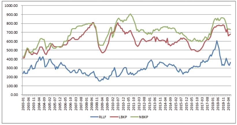
https://cdn.apub.kr/journalsite/sites/ktappi/2019-051-05/N0460510504/images/JKTAPPI_2019_v51n5_38_f001.jpg

Fig. 1.

Movements of the wood pulp (LBKP, NBKP) price and CME random length lumber futures (RLLF) price, January 2003 through June 2019.

3.1 Results of unit root tests

Table 1 presents the results of the ADF test to determine the presence of a unit root in the prices of wood pulp (LBKP and NBKP) and CME RLLF. While the null hypothesis of a unit root (or non-stationarity) can not be rejected in price levels, the ADF test performed on the first differences indicates that the first difference of each series is stationary. The results confirm that both the wood pulp and CME lumber futures price series are difference stationary, or I(1), integrated of order one.

Table 1.

Results of unit root tests

Variable	ADF-statistic	Critical Value
Price Levels
LBKP_t	-3.67	-4.01
NBKP_t	-3.11	-4.01
RLLF_t	-2.75	-4.01
First Differences
ΔLBKP_t	-6.10**	-3.46
ΔNBKP_t	-9.45**	-3.46
ΔRLLF_t	-11.81**	-3.46

1) ** indicates statistical significance at the 1% level.

3.2 Results of Johansen cointegration tests

Table 2 reports the results of Johansen cointegration tests for two pairs of price series, in other words, LBKP vs. RLLF, and NBKP vs. RLLF. The maximum eigenvalue (λ_max) statistics indicate that the null hypothesis of r=0 (no cointegration) cannot be rejected at the 5% significance level. The results show evidence of zero cointegrating vector between the two price series, suggesting that there exists no cointegration or long-run equilibrium relationship between the wood pulp (LBKP and NBKP) and CME RLLF.

Table 2.

Results of Johansen cointegration tests

LBKP vs. RLLF				NBKP vs. RLLF
H₀	H_A	λ_max	Critical value	H₀	H_A	λ_max	Critical value
r=0	r=1	12.13	14.26	r=0	r=1	10.22	14.26
r=1	r=2	3.99	3.84	r=1	r=2	4.21	3.84

1) Critical values are obtained from MacKinnon et al.⁵⁾

3.3 Results of vector autoregressive (VAR) model and granger causality

Table 3 presents the results of the vector autoregressive (VAR) model between LBKP and RLLF, and Granger causality test. On the left-hand side of Table 3, the coefficients of lagged terms ΔRLLF_t-j are not statistically significant at all. The result indicates that the lumber futures market does not lead the wood pulp (LBKP) market in the lead-lag relationships. The Granger causality test also fails to reject the null hypothesis that RLLF does not Granger cause LBKP.

Table 3.

Results of vector autoregressive (VAR) model and granger causality

(LBKP vs. RLLF)

Variable	ΔLBKP_t		ΔRLLF_t
Variable	Coefficient	t-statistic	Coefficient	t-statistic
Intercept	24.0770	2.06*	64.6475	2.53*
ΔLBKP_t-1	1.3136	19.52**	0.1787	1.22
ΔLBKP_t-2	-0.3606	-5.43**	-0.2264	-1.56
ΔRLLF_t-1	0.0310	0.95	1.1179	15.74**
ΔRLLF_t-2	-0.0201	-0.62	-0.1778	-2.51*
Granger causality test	F-statistic	P-value	F-statistic	P-value
	H₀: RLLF does not Granger cause LBKP		H₀: LBKP does not Granger cause RLLF
	0.8923	0.4114	2.0153	0.1361

1) * and ** indicate statistically significant at the 5% and 1% level respectively.

On the right-hand side of Table 3, the coefficients of lagged terms ΔLBKP_t-i are not statistically significant, and the Granger causality test also fails to reject the null hypothesis that LBKP does not Granger cause RLLF at the 5% significance level. The results generally show that Granger causality runs in no direction between LBKP and CME RLLF.

Table 4 presents the results of vector autoregressive (VAR) model between NBKP and RLLF, and Granger causality test. The results are exactly the same with those of VAR model between LBKP and RLLF, presented in Table 3. The results presented in Tables 3-4 suggest that the wood pulp and CME random length lumber futures are independent and there exists no correlation between them.

Table 4.

Results of vector autoregressive (VAR) model and granger causality

(NBKP vs. RLLF)

Variable	ΔNBKP_t		ΔRLLF_t
Variable	Coefficient	t-statistic	Coefficient	t-statistic
Intercept	24.9592	2.30*	56.4672	2.25*
ΔNBKP_t-1	1.3220	19.70**	-0.0094	-0.06
ΔNBKP_t-2	-0.3667	-5.57**	-0.0279	-0.18
ΔRLLF_t-1	0.0165	0.54	1.1251	15.75**
ΔRLLF_t-2	-0.0089	-0.29	-0.1814	-2.55*
Granger causality test	F-statistic	P-value	F-statistic	P-value
	H₀: RLLF does not Granger cause NBKP		H₀: NBKP does not Granger cause RLLF
	0.4052	0.6674	0.6403	0.5283

1) * and ** indicate statistically significant at the 5% and 1% level respectively.

3.4 Results of estimating cross hedge ratio and hedging effectiveness

Table 5 presents the results of the linear regression model estimated to obtain the risk-minimizing cross hedge ratio and hedging effectiveness. The estimated slope coefficients (β₁) are 0.0112, 0.0194 respectively, and their correspondent t-statistics show that the estimated hedge ratios are not statistically significant. This implies that the movements in CME RLLF prices cannot explain the movements in wood pulp (LBKP and NBKP) prices.

Table 5.

Results of estimating cross hedge ratio and hedging effectiveness

Variable	No. of Obs.	β₀	β₁	R²
ΔLBKP_t vs. ΔRLLF_t	197	0.2483 (0.93)	0.0112 (0.32)	0.0005
ΔNBKP_t vs. ΔRLLF_t	197	0.2645 (1.04)	0.0194 (0.59)	0.0018

1) Numbers in parenthesis represent t-statistics.

On the other hand, R²s are 0.0005, 0.0018 respectively, indicating that the variation in wood pulp (LBKP and NBKP) prices is little explained by the variation in CME RLLF prices. The result suggests that the variation in wood pulp prices accounted for by the estimated regression model is not significant.

The above results, in general, suggest that CME RLLF cannot be used as a cross hedging vehicle for wood pulp. The results could be somewhat foreseen considering the distinct differences between wood pulp and CME lumber in terms of tree species (hardwood vs. softwood), usage (paper production vs. residential home construction), and the like.

4. Conclusions

The primary goal of this study is to determine the cross hedging potential of CME RLLF for wood pulp. The Johansen cointegration tests showed that wood pulp and CME lumber futures were not cointegrated. This suggests that there is no long-run equilibrium relationship between them. The results from Granger causality tests showed no evidence of a causal relationship between wood pulp and CME RLLF. This implies that there is no correlation between them. The results of the regression model also showed that the estimated hedge ratios were not statistically significant and the variation in wood pulp prices was not well explained by the variation in CME RLLF prices. As a conclusion, CME RLLF cannot be used effectively as a cross hedging vehicle for wood pulp.

Footnotes

[6] [1] Thus far, there have been several attempts to launch futures contracts on wood pulp around the world, but all ended up in failure.¹⁾ Most recently, the CME Group launched a softwood pulp futures contract in September 2007. The exchange launched a hardwood pulp futures contract in January 2009 as well.²⁾ Both contracts were permanently delisted in 2012 due to the lack of liquidity (trading volume). The pulp and paper industry is probably the last of the major commodity markets without a functioning futures exchange where hedging would be carried out.

[7] [2] Cross hedging is used when the same futures contract is not available on the commodity being hedged. A futures contract that is similar, but not identical to the underlying commodity, with a high degree of price correlation is used as a substitute.

[8] [3] The contract unit for CME random length lumber futures is 110,000 board feet, and the price is quoted in dollars per 1,000 board feet (mbf). The minimum tick size is $0.10 per 1,000 board feet (=$11.00/contract). The contract months are January, March, May, July, September and November. The last trading day is the business day prior to the 16th calendar day of the contract month. The trading hours are from 9:00 a.m. to 3:05 p.m. central time, Monday through Friday. The final settlement is done by physical delivery. The delivery unit of each lumber contract consists of 2 inches thick by 4 inches wide, with random lengths ranging from 8 to 20 feet. The primary deliverable lumber species is Western Spruce-Pine-Fir (SPF) including Hem-Fir, Engelmann Spruce and Lodgepole Pine. The producing mills must be located in the states of Oregon, Washington, Idaho, Wyoming, Montana, Nevada, California, or the Canadian provinces of British Columbia or Alberta.

[9] [4] The following tests are conducted using the software package EViews 10.

[10] [5] The optimal lag length m was determined using the Akaike Information Criterion (AIC).

Literature Cited

Till, H., Why haven’t pulp futures contracts succeeded? A case study, Journal of Governance and Regulation 4(4):515-523 (2015).

10.22495/jgr_v4_i4_c4_p9

CME Group, Softwood and Hardwood Pulp Futures and Options, Chicago, USA (2009).

Johansen, S., Estimation and hypothesis testing of cointegration vectors in gaussian vector autoregressive models, Econometrica 59:1551-1580 (1991).

10.2307/2938278

Ederington, L. H., The hedging performance of the new futures markets, Journal of Finance 34:157-170 (1979).

10.1111/j.1540-6261.1979.tb02077.x

MacKinnon, J. G., Haug, A. A., and Michelis, L., Numerical distribution functions of likelihood ratio tests for cointegration, Journal of Applied Econometrics 14:563-577 (1999).

10.1002/(SICI)1099-1255(199909/10)14:5<563::AID-JAE530>3.3.CO;2-I

Journal of Korea TAPPI ISSN:0253-3200(Print) 펄프종이기술

Preview

The Feasibility of Cross Hedging Wood Pulp with CME Lumber Futures

ABSTRACT

MAIN

[1]

[2]

[3]

[4]

[5]

[6]

[7]

Fig. 1.

Movements of the wood pulp (LBKP, NBKP) price and CME random length lumber futures (RLLF) price, January 2003 through June 2019.

Table 1.

Results of unit root tests

Table 2.

Results of Johansen cointegration tests

Table 3.

Results of vector autoregressive (VAR) model and granger causality

Table 4.

Results of vector autoregressive (VAR) model and granger causality

Table 5.

Results of estimating cross hedge ratio and hedging effectiveness

Footnotes

Literature Cited