A Non-Contact Method for Real-Time Stacked Sheets Counting with X-ray Absorption Spectra and Long Short-Term Memory Network

Zheng Fang; Bingan Yuan; Mengyi Wang; Bichao Ye; Shunren Li; Yinbin Chen; Hongjun Deng; Shucheng Feng; Kun Qian

doi:10.7584/JKTAPPI.2023.6.55.3.3

Preview

Original Paper

Journal of Korea TAPPI. 30 June 2023. 3-14
https://doi.org/10.7584/JKTAPPI.2023.6.55.3.3

A Non-Contact Method for Real-Time Stacked Sheets Counting with X-ray Absorption Spectra and Long Short-Term Memory Network

Zheng Fang¹^†

Bingan Yuan²

Mengyi Wang³

Bichao Ye³

Shunren Li⁴

Yinbin Chen⁵

Hongjun Deng⁵

Shucheng Feng⁵

Kun Qian⁵

¹School of Aerospace Engineering, Xiamen University, Xiamen 361102, P.R. China, Professor

²School of Aerospace Engineering, Xiamen University, Xiamen 361102, P.R. China, Doctoral Student

³School of Aerospace Engineering, Xiamen University, Xiamen 361102, P.R. China, Graduate Student

⁴ASR Technology (Xiamen) Co., Ltd., Xiamen 361021, P.R. China, Chief Executive Officer

⁵School of Aerospace Engineering, Xiamen University, Xiamen 361102, P.R. China, Undergraduate Student

^†Corresponding author: E-Mail: fangzheng@xmu.edu.cn (Address: School of Aerospace Engineering, Xiamen University, Xiamen 361102, P.R. China)

ABSTRACT

Stacked sheets counting is an important segment in the printing and packaging industry. It can meet the strict quality control and avoid great economic loss. Traditional counting methods based on photoelectric sensors or image processing face the challenges of low efficiency, breakage, and low contrast. In this paper, a non-contact and real-time counting method was developed by combining broadband X-ray absorption spectra (XAS) with long short-term memory network (LSTM). First, 500 sheets of standard A4 (70 g/m²) printing paper stacked one by one were scanned by the broadband XAS detection equipment. Second, the collected 500 broadband XAS data were pre-processed by principal component analysis (PCA) to reduce the data dimension. Finally, LSTM was constructed to extract the temporal features of XAS data and establish a relationship with the number of paper sheets; meanwhile, polynomial fitting model(PFM) and artificial neural network (ANN) were proposed to compare with LSTM. The results showed that the combination of broadband XAS and LSTM had a maximum error of 1.8504 sheets and a single measurement time of 0.006 sec. To the best of our knowledge, this work was the first study to analyze and utilize the broadband XAS and LSTM for counting task. It provided a new non-contact and real-time counting method for stacked sheets.

Keywords

Stacked sheets counting

X-ray absorption spectra

principal component analysis

long short-term memory network

MAIN

1. Introduction
2. Materials and Methods
2.1 Materials
2.2 Methods
3. Results and Discussion
3.1 Analysis of X-ray spectra
3.2 Data dimension reduction and partition
3.3 Model evaluation indexes
3.4 Result visualization analysis
4. Conclusions

1. Introduction

Stacked sheets counting is an important operation in paper and printing industry, such as the in-line binding process of book printing, high-level printing and security labeling fields.¹⁾ The traditional manual counting methods by measuring the physical attributes of a pack, obtaining the total and average parameters of weight or height, and the number of stacks can be obtained by division. Manual counting is the most primitive counting method, which is extremely tedious and can lead to counting errors due to the individual attribute differences.²⁾ Some in-line contact technologies can also be used for paper thickness measurement, such as magnetic reluctance and eddy current sensors. Magnetic sensors can provide kHz sampling rate and high accuracy up to micrometer precision. However, they need to contact on both sides of the paper and compress stacks under a fixed pressure,³⁾ worse still, the paper can be easily damaged by these mechanical operations.⁴⁾ In general, these traditional methods have the disadvantages of low efficiency, breakage and inaccurate counting.

Some non-contact measurement methods have been applied to stacked sheets counting in recent years. They can be divided into two categories: based on machine vision technology and using radioactive rays. In the method of machine vision, Sato, J. et al. detect the boundaries of stacked facial oil blotting papers for counting,⁵⁾ but this method can be confused with the paper boundary and crease. Han, X. et al. propose a stacked paper counting approach based on image texture.⁶⁾ However, this approach is only suitable for regular stacks, which is difficult to apply in practical production. Zhu, H. et al. build a counting system for ultra-high stacks,where the camera array is used to capture the edge texture images of the packed papers.⁷⁾ Xiao, C. et al. use local histogram equalization algorithm and bi- Gaussian linear enhancement algorithm to detect the low contrast images of stacked white paper sheets.⁸⁾ However, it needed a priori knowledge of the template size for histogram equalization. The above detection methods require the sheets to be stacked regularly, i.e., the edge characteristics of each substrate must be shown. In addition, these methods are not suitable for stacked sheets with transparent material, rough edge, low edge resolution, too thin substrate, and sticking sheets, as the contour features cannot be clearly shown in these situations. Zhao, H. et al. design a stripe detection method, using local template matching algorithm and a global frequency domain filtering algorithm.⁹⁾ This approach can accurately count when the substrates are distorted and irregularly stacked. Pham, D. et al. use a U-Net network for the segmentation and counting of stacked sheets,¹⁰⁾ and this method can solve the interference caused by rough edges, low edge resolution, and adhering sheets. However, there are still some challenges that cannot be overcome, such as transparent substrates, hidden sheets, and sheets that are too thin.

In the radioactive ray measurement, the X-ray thickness gauge is commonly used. When the X-ray penetrates objects of different thickness(d), the detector receives different X-ray intensities(I), the object is thicker, the received X-ray intensity is weaker, taking advantage of this property, the thickness of the object can be obtained.¹¹⁾ However, there’s no model that can well build the relationship between d and I. Shi, Y proposes a liner interpolation model for gamma ray thickness gauge,¹²⁾ but the accuracy of the model depended on the number of calibration plate. As the number of plate increased, the calibration time increased dramatically. Unlike the gamma rays, which are mono-energetic ray, the multi-energetic X-ray suffer from hardening phenomenon in the transmission process. Xu, G. et al. develop a non-linear model to fit the X-ray attenuation process,¹³⁾but there is an estimation error in solving the model parameters. Generally, a five degree polynomial model is used in X-ray thickness gauge.¹⁴⁾ However, for a large measurement range, it needs piece-wise fitting to reduce the model’s error. Additionally, the total thickness of calibration plates should cover the whole measurement range.

Based on the above problems, a fast in-line counting method based on photon counting detector (PCD) was proposed. 500 A4 papers were prepared to collect X-ray absorption spectra (XAS) data. After the data were preprocessed by principal component analysis (PCA), three counting models were constructed: polynomial fitting model (PFM), artificial neural network (ANN) and long short-term memory network (LSTM). The main data features extracted by PCA were used to train these models.

2. Materials and Methods

2.1 Materials

2.1.1 Instruments and data acquisition

The schematic diagram of the broadband XAS detection equipment was shown in Fig. 1. This equipment was designed by our laboratory.¹⁵⁾ The lead shell of the equipment could avoid X-ray radiation leakage, and the experimental samples were isolated from the external environment.

https://cdn.apub.kr/journalsite/sites/ktappi/2023-055-03/N0460550301/images/ktappi_55_03_01_F1.jpg

Fig. 1.

Schematic diagram of the XAS detection equipment.

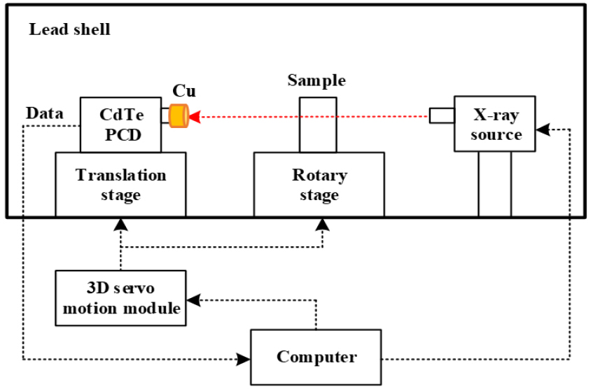
The core components of the detection equipment included a three-dimensional (3D) servo motion module, an X-ray source, and a CdTe photon counting detector (PCD). The 3D servo motion module could control the translation of the PCD and the rotation of the rotary table. The cone beam X-ray source was manufactured by American MOXTEK Company, and its model number was 60 kV-12 W MAGPRO. This X-ray source was a tungsten target X-ray tube, and the tube voltage range was 4-60 kV, the tube current range was 0-1000 μA, the focal size was 400 μm, and the maximum power was 12 W. Through the translation stage, the PCD could be adjusted on the same line. The rotary stage could fine-tune stacked sheets so that they were vertical with the X-ray source.

The CdTe PCD was manufactured by American Amptek Company, and its model number was X-123. The PCD was a semiconductor detector with an energy resolution of <1.2 keV. The photon energy channels of CdTe PCD were separated, and the number of photons in each photon energy channel was obtained. The PCD had 512 photon energy channels, and the calibration relationship of photon channel and energy was given by Eq. 1.¹⁵⁾

[1]

E = 200.7639 \times (n - 0.3561)

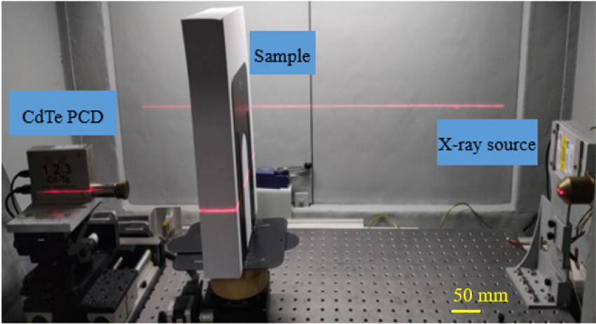
where, n was the photon channel, E (eV) was the photon energy. A collimator (Cu cap, outer diameter 24 mm) was used to remove the scattered X-ray photons. The sample and experimental platform were shown in Fig. 2. The sample was placed 125 mm from the PCD and 475 mm from the X-ray source. A fan-beam laser of 650 nm wavelength was used to indicate the center of the X-ray source and the Be window of the PCD to ensure that they were at the same level.

https://cdn.apub.kr/journalsite/sites/ktappi/2023-055-03/N0460550301/images/ktappi_55_03_01_F2.jpg

Fig. 2.

The sample and experimental platform.

According to relative works,¹⁶⁾ and through extensive tests, the X-ray tube voltage was set at 40 kV and the X-ray tube current was set at 8 μA, and each X-ray spectrum was measured for 30 s. Five hundred sheets of standard A4 printing paper (70 g/m²) were taken as experimental samples, and the papers were produced by Deli Company. To reduce the differences in individual characteristics, these papers were from the same package, so the production and storage environments were similar. Finally, the X-ray transmission spectra of 1 to 500 sheets of paper were measured.

2.1.2 XAS data preparation and preprocessing

When a single-energy X-ray of incident intensity I₀ penetrated a homogeneous medium of thickness d, the X-ray intensity was attenuated to I. The attenuation process could be described by the Beer- Lambert law,¹⁷⁾ and was given by Eq. 2:

[2]

I = I_{0} e^{(- u d)}

where, u was the X-ray attenuation coefficient, which was related to X-ray absorption and scattering effects. However, X-ray scattering effect could be negligible in this experiment. On the one hand, due to the PCD received data were composed with hundreds of channels and analyzed as an integration. The distorted XAS data caused by scattering effect were inputted into the models (details in section 2.2), which learnt the non-linear relationship between XAS and stacked sheets number. The scattered photons in multiple channels could not have an obvious affection on the results, especially for the proposed neural network models. On the other hand, the scattering occurred little as the penetrated stacked paper sheets (main components were carbon, hydrogen, and oxygen) had a low atomic number. Therefore, the X-ray absorption coefficient μ could be calculated by Eq. 3.

[3]

u = \frac{1}{d} \ln (\frac{l_{0}}{I})

The X-ray photon measured by PCD was approximated as monoenergetic X-ray in each photon energy channel. The X-ray absorption coefficient in each photon energy channel was calculated from the incident and transmitted X-ray spectrum, and the broadband XAS in a certain photon energy range was obtained. Eq. 3 showed that the sample’s thickness d was related to attenuation index u at a given incident X-ray energy. Therefore, stacked sheets counting could be achieved theoretically.

In this experiment, 500 X-ray incident spectra and transmitted spectra were measured, and the broadband XAS were calculated via Beer-Lambert law. Then, the XAS data were normalized to 0–1 in order to eliminate the interference of singular data. In addition, normalization could accelerate gradient descent for getting the optimal solution of the model.¹⁸⁾

As the original XAS data had 165 features, which were an overload for the lightweight model and not suitable for real-time processing. Common data dimension reduction techniques include: linear discriminant analysis (LDA),¹⁹⁾ factor analysis (FA),²⁰⁾ principal component analysis (PCA),²¹⁾ and singular value decomposition (SVD).²²⁾ Since PCA was a relatively simple and effective dimension reduction method, so it was used to reduce the dimension of XAS data. Sample of XAS data X as example:

[4]

X = [x_{1}, x_{2}, \dots, x_{D}]

where, $D = 165$ , then compressed each feature as follows:

[5]

x_{i} = x_{i} - \frac{1}{D} \sum_{i = 1}^{D} x_{i}

Calculating the covariance matrix $X X^{T}$ and do eigenvalue decomposition, ranking the eigenvalues from large to small, taking the largest eigenvector $w_{d}$ of the first d eigenvalues to form the feature transformation matrix W:

[6]

W = [w_{1}, w_{2}, \dots, w_{d}]

Finally, the principal component of the initial XAS data could be represented by P:

[7]

P = W^{T} X

Using P as a replacement for the original XAS data, the data dimension was reduced, and most of the content could be retained.

2.2 Methods

Three models were constructed to establish a relationship between the pre-processed XAS data and the number of stacked sheets, and the performance of these models was compared.

2.2.1 Polynomial fitting Model

Polynomial fitting model (PFM) was widely used in X-ray thickness gauge,¹¹⁾ it could be written as Eq. 8.

[8]

d = \sum_{(i = 0)}^{n} a_{i} (\ln I)^{i}

where d was the thickness of the object, and I was the transmitted X-ray intensity. In this experiment, d was the number of stacked sheets, and I was the number of X-ray photons received by the PCD. The index n was important for model’s accuracy, and should be chosen carefully. A smaller degree led to a lower fitting accuracy, a larger degree could get a better result but increased the complexity of the calibration. To achieve a balance between model accuracy and calibration effort, the polynomial degree was set to five.¹⁴⁾

2.2.2 Artificial neural network

An artificial neural network (ANN) model was constructed to establish a relationship between XAS data and stacked sheet thickness. ANN was composed of many neurons, and in theory, a neural network with a single hidden layer containing a finite number of neurons and a nonlinear activation function could fit any nonlinear function.^23,24) The structure of ANN mainly included input layer, multi- hidden layers, and output layer. It consisted of many functions like Eq. 9:

[9]

y_{i} + 1 = f (\sum_{i} w_{i} x_{i} - b_{i})

where $f (x)$ was the activation function of the hidden layer, $w_{i}$ was the weight of the neuron node, and $b_{i}$ was be offset.

As XAS data belonged to 1 dimension (1D) data and its complexity was reduced by PCA, so the network was constructed with only two dense layers. This could capture the features of XAS data and avoid overfitting. Rectified linear unit (Relu) was a kind of nonlinear activation function that could avoid vanishing gradient and exploding gradient, it was shown as the following formula:

[10]

R e l u (x) = \max (0, x)

The nonlinear activation function sigmoid was also known as the logistic function, which could map the data between 0 and 1. Sigmoid could be expressed as:

[11]

S i g m o i d (x) = \frac{1}{1 + e^{- x}}

Relu was taken as the activation function of the hidden layer, sigmoid was taken as the activation function of the output layer. The optimized values of the main hyper-parameters of the ANN were shown in Table 1.

Table 1.

The optimized values of ANN hyper- parameters

Hyper-parameter	Optimized value
Optimizer	Adam
Activation function of hidden layer	ReLU
Activation function of output layer	Sigmoid
Learning rate	0.001
Batch size	16
Max iteration	100
Loss function in training	MSE
Number of hidden layers	2
Number of nodes in each hidden layer (in order)	32, 32

2.2.3 Long short-term memory network

As XAS data is one dimensional data, and in stacked sheets counting scenes such as book binding and paper packaging, the paper sheets were stacked one by one, the current XAS data was related to the previous stacked sheets. Therefore, to a certain extent, the XAS data had temporal sequence property. Long short term memory network (LSTM) is good at addressing 1D data especially those with temporal properties.²⁵⁾ It can selectively retain the information of previous layers. The structure of LSTM was depicted in Fig. 3. It consisted of many timestep. Taking the t timestep as an example, namely the middle block in the model, there were three inputs and two outputs, the input $c_{t - 1}$ was the cell state information of t-1 timestep, the input $h_{t - 1}$ was the output of t-1 timestep, and the input $X A S_{t} \dots X A S_{t + s e q}$ was the input of t timestep, namely the XAS data sequence. It meant that using the XAS data from $t$ to $t + s e q$ timestep to predict the number of stacked sheets at $t + s e q + 1$ timestep. The output $c_{t}$ was the reserved state information of t timestep and $h_{t}$ was the output of current timestep. Noted that all the input and output variables were vectors. The internal computations in the t timestep were as follows:

[12]

(\begin{matrix} f_{t h} \\ i_{t h} \\ o_{t h} \\ \tilde{c_{t}} \end{matrix}) = (\begin{matrix} σ \\ σ \\ σ \\ \tanh \end{matrix}) [W (\begin{matrix} X A S_{t} \dots X A S_{t + s e q} \\ h_{t - 1} \end{matrix}) + B]

where, $w = (\begin{matrix} w_{f} \\ w_{i} \\ w_{o} \\ w_{tahn} \end{matrix}), B = (\begin{matrix} b_{f} \\ b_{i} \\ b_{o} \\ b_{c} \end{matrix})$

$c_{t}$ and $h_{t}$ could be calculated as:

[13]

c_{t} = f_{t h} ･ c_{t - 1} + i_{t h} ･ \tilde{c_{t}}

[14]

h_{t} = o_{t h} ･ \tanh (c_{t})

where $f_{t h}$ was called forget gate. It decided the probability of preserving the information of the last timestep $h_{t - 1}$ . As it was caculated by sigmoid activation function 𝜎, it belonged to [0, 1]. How much of the current timestep’s information was contained depending on the input gate $i_{t h}$ and the current input information $\tilde{c_{t}}$ . The activation functions were sigmoid and tanh respectively, and the current timestep reserved state information screened by Eq. 13. The final output $h_{t}$ was calculated in Eq. 14, which was decided by the output gate $o_{t h}$ . The gate selected how much content should be released at this timestep, the $o_{t h}$ was also activated by sigmoid function.

https://cdn.apub.kr/journalsite/sites/ktappi/2023-055-03/N0460550301/images/ktappi_55_03_01_F3.jpg

Fig. 3.

LSTM architecture.

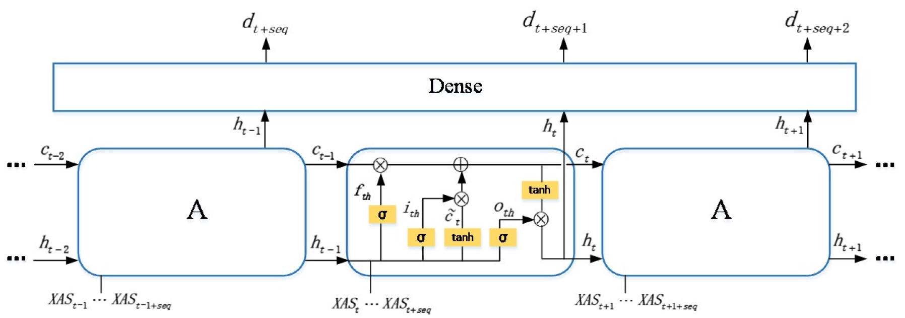
The current timestep’s output $h_{t}$ (multi-dimensional vector) was inputted to the next dense layers, which gradually converged the multi-dimensional data ( $h_{t}$ ) to one dimension, namely the number of stacked paper sheets. The optimized hyperparameters of LSTM were shown in Table 2.

Table 2.

The optimized values of LSTM hyper- parameters

Hyper-parameter	Optimized value
Optimizer	Adam
Length of timestep sequence	10
Number of nodes in LSTM output space	100
Number of nodes in each dense layer (in order)	40, 1
Learning rate	0.0001
Batch size	30
Max iteration	100
Loss function in training	MSE

3. Results and Discussion

3.1 Analysis of X-ray spectra

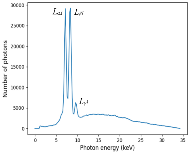
In this experiment, the X-ray tube voltage was set at 40 kV and the X-ray tube current was set at 8 μA after extensive experiments. The measured X-ray incident spectrum was shown in Fig. 4. There was no sample placed on the rotary table. Tungsten (⁷⁴W) was the anode (target) material for the X-ray source, and the incident spectrum was the L-series excitation spectrum of tungsten. In Fig. 4, The y-coordinate was the number of X-ray photons measured by the CdTe PCD, and the x-coordinate was the photon energy. The incident spectrum had three characteristic peaks of L_α1, L_β1, and L_γ1, and the photon energy of the peaks were L_α1 = 8.3976 keV, L_β1 = 9.6724 keV, L_γ1 = 11.2859 keV.

https://cdn.apub.kr/journalsite/sites/ktappi/2023-055-03/N0460550301/images/ktappi_55_03_01_F4.jpg

Fig. 4.

X-ray incidence spectrum of X-ray tube at 40 kV, 8 μA.

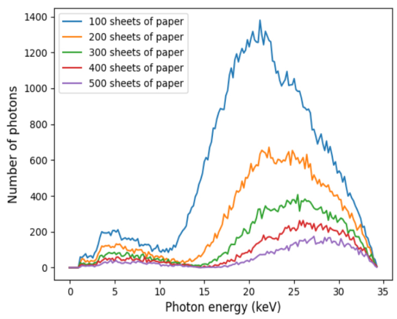
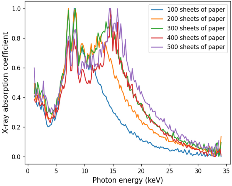
Since the numbers of stacked papers were up to 500, only the X-ray transmission spectra and XAS of 100 sheets, 200 sheets, 300 sheets, 400 sheets and 500 sheets were plotted in Fig. 5 and Fig. 6. They showed that there were obvious discrepancies in the XAS for different numbers of stacked papers, especially in the photon energy range from 10 keV to 34 keV. With the differences existing in the XAS of different numbers of stacked papers, the proposed models could build the relationship between XAS data and stacked papers.

https://cdn.apub.kr/journalsite/sites/ktappi/2023-055-03/N0460550301/images/ktappi_55_03_01_F5.jpg

Fig. 5.

The X-ray transmitted spectra of 100 sheets, 200 sheets, 300 sheets, 400 sheets and 500 sheets.

https://cdn.apub.kr/journalsite/sites/ktappi/2023-055-03/N0460550301/images/ktappi_55_03_01_F6.jpg

Fig. 6.

The XAS of 100 sheets, 200 sheets, 300 sheets, 400 sheets and 500 sheets.

3.2 Data dimension reduction and partition

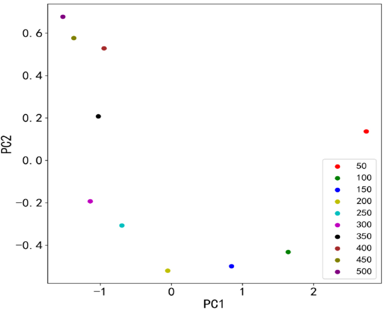
As discussed in 2.1.2, the PCA algorithm was used to reduce the dimension of XAS. The contribution rate and cumulative contribution rate (CCR) were shown in Table 3. It showed that the CCR of the top 5 principal components reached 96.56% (>95%,²⁶⁾), which meant that if the top 5 principal components were used to substitute the original XAS data, then 96.56% of the original content could be remained. The distributions of the top 2 principal components were shown in Fig. 7. These results showed that the top 2 principal components could effectively discriminate between different numbers of stacked sheets. In this experiment, the top 5 principal components were taken as input of the three models.

Table 3.

Contribution rate and cumulative contribution rate of the top 5 principal components

Principal component	Contribution rate (%)	Cumulative contribution rate (%)
PC1	79.88	79.88
PC2	7.81	87.69
PC3	4.97	92.66
PC4	2.82	95.48
PC5	1.08	96.56

https://cdn.apub.kr/journalsite/sites/ktappi/2023-055-03/N0460550301/images/ktappi_55_03_01_F7.jpg

Fig. 7.

Distribution of the top 2 principal components.

For the ANN and LSTM models, 10% of the data set was randomly selected as the test set, and the remaining 90% of the data set was randomly divided into a training set and validation set with a ratio of 9:1. The PFM was fitted using the method in.¹³⁾ According to Eq. 8, each pair of fitting points (d, I) consisted of the sheets number d and the transmitted X-ray density I. The fitting points including the minimum, maximum and other points were evenly distributed in all 500 stacked sheets, and the PFM was tested on the rest points. The training computer was configured with 16 CPU cores (2.9GHz, i7-10700F), 32GB RAM and a GPU (NVIDIA GeForce RTX3060).

3.3 Model evaluation indexes

Mean square error (MSE), mean absolute error (MAE), max absolute error (MAXE) and Coefficient of determination (R²) were selected as evaluation indexes of the above models. MSE and MAE recorded the prediction accuracy in different dimensions. MAXE reflected the worst prediction accuracy of the model. The smaller values of MSE, MAE and MAXE led to the higher fitting accuracy of the model. R² recorded the overall fitting accuracy of the model, and the value of R² ranged from -∞ to 1. The closer R² was to 1, the better the fit. The evaluation indexes were shown in Eqs. 15, 16, 17, 18.

[15]

M S E (y, \hat{y}) = \frac{1}{n} \sum_{i = 0}^{n - 1} (y_{i} - {\hat{y}}_{i})^{2}

[16]

M A E (y, \hat{y}) = \frac{1}{n} \sum_{i = 0}^{n - 1} |y_{i} - {\hat{y}}_{i}|

[17]

M A X E (y, \hat{y}) = \max |y_{i} - {\hat{y}}_{i}|

[18]

R^{2} (y, \hat{y}) = 1 - \frac{\sum_{i = 1}^{n} (y_{i} - {\hat{y}}_{i})^{2}}{\sum_{i = 1}^{n} (y_{i} - \bar{y})^{2}}

where n was the total number of test set, $y_{i}$ and ${\hat{y}}_{i}$ were the true and predicted values of the i-th data respectively, and $y$ was the mean value of $y_{i}$ .

3.4 Result visualization analysis

The MSE, MAE, MAXE, and R² of PFM, ANN and LSTM were shown in Table 4, and the bold values were the better results among these models. It showed that all the index results of LSTM were better than those of PFM and ANN. However, the results of PFM were better than ANN. It may be the PFM was fitted by five degree polynomial, which was more expressive than ANN (fitted by two fully connected layers). The errors between the actual number of stacked papers and the predicted values by PFM were drawn in Fig. 8. The horizontal axis represented the log value of X-ray transmission intensity, and the greater transmission intensity represented the less stacked papers had been penetrated. As shown in Fig. 8, the predicted values agree well with the actual values when the stacked sheets were more than 20. However, when the penetrated papers decreased, the PFM could not get a good performance. This was because the thinner samples the less X-ray attenuation could be detected, so there were less differences between incident and transmitted X-ray intensity, which was important for the accuracy of PFM.

https://cdn.apub.kr/journalsite/sites/ktappi/2023-055-03/N0460550301/images/ktappi_55_03_01_F8.jpg

Fig. 8.

The fitting performance of PFM.

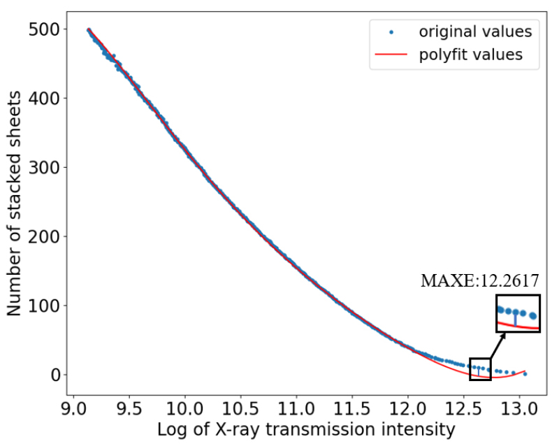
Table 4.

The index results of PFM, ANN and LSTM

Model	MSE (sheet)	MAE (sheet)	MAXE (sheet)	R²
PFM	9.4004	2.1032	12.2617	0.9995
ANN	35.5828	3.5656	22.4591	0.9981
LSTM	0.5236	0.5197	1.8504	0.9999

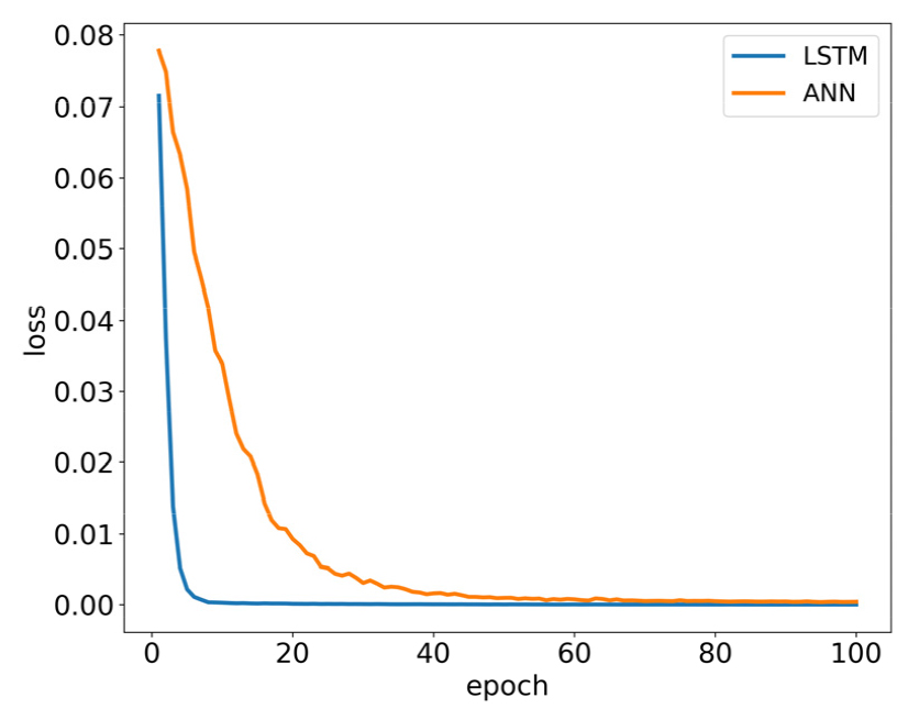
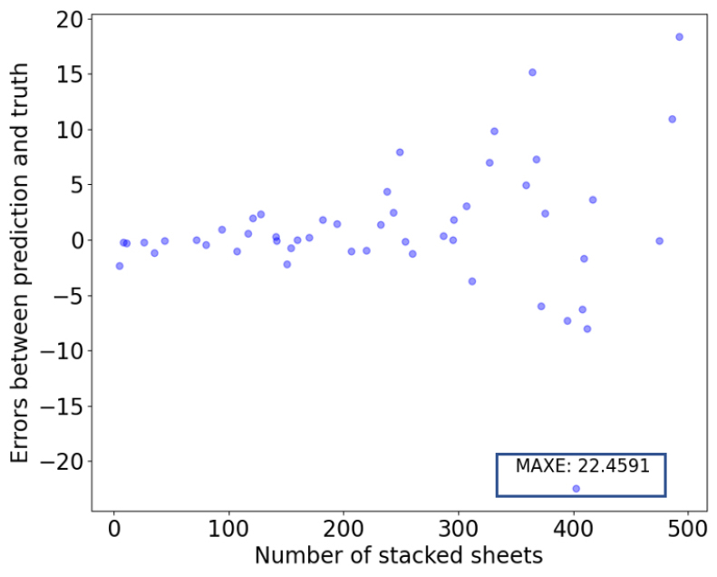
The two artificial neural networks (ANN and LSTM) built non-linear relationships between XAS data and stacked sheets. The training processes of the models were shown in Fig. 9. It could be seen that LSTM converged faster than ANN, and the loss curve of LSTM was also below that of ANN. It meant that the proposed LSTM model was more suitable for this task than ANN. This could also be evidenced in Fig. 10 and Fig. 11. From the results of the two models, we could intuitively find that the errors of ANN were much larger than that of LSTM. In the test data of ANN, the MAXE 22.4591 occurred when the number of stacked sheets was 402. The negative value meant that the predicted value was less than the true value, and the MAXE of LSTM was 1.8504, which occurred when the number of stacked papers was 444 sheets.

https://cdn.apub.kr/journalsite/sites/ktappi/2023-055-03/N0460550301/images/ktappi_55_03_01_F9.jpg

Fig. 9.

The training loss of ANN and LSTM.

https://cdn.apub.kr/journalsite/sites/ktappi/2023-055-03/N0460550301/images/ktappi_55_03_01_F10.jpg

Fig. 10.

Scatter plot of prediction error of ANN.

https://cdn.apub.kr/journalsite/sites/ktappi/2023-055-03/N0460550301/images/ktappi_55_03_01_F11.jpg

Fig. 11.

Scatter plot of prediction error of LSTM.

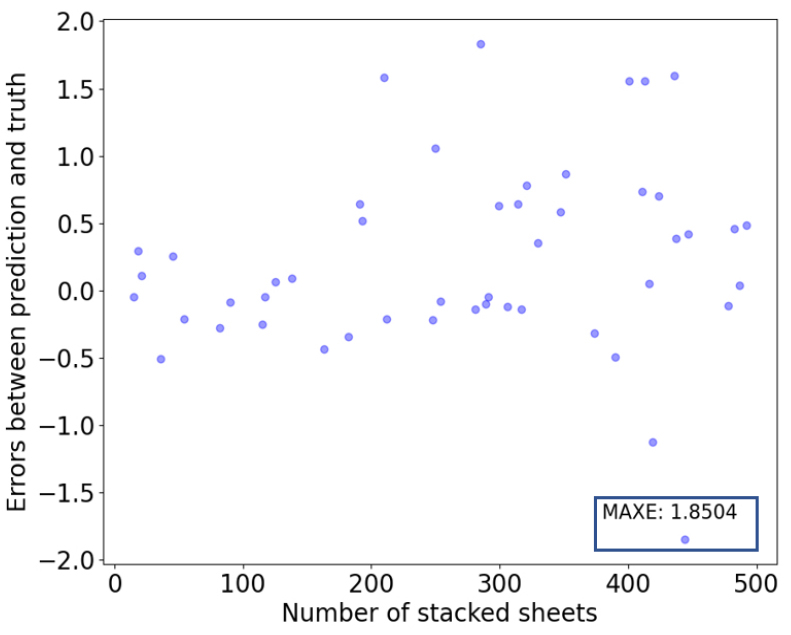
From the above analysis, we could see that the accuracy of these two neural networks was not affected by thinner stacked sheets, which was different from PFM. For the both two models, the prediction errors of the thinnest stacked sheets were smaller than those of the thickest stacked sheets.

Compared with the commonly used PFM in X-ray thickness measurement, the combination of XAS with neural networks (ANN and LSTM) took full advantage of absorption attenuation in separate energy channels, and the XAS relied not only on the transmitted X-ray intensity but also on the incident intensity, so it was less sensitive to the tube current change of the X-ray source and more robust than the traditional X-Ray thickness measurement, which only depended on the transmitted X-ray intensity. Additionally, PFM needed to calibrate the whole measuring range and even needed piece-wise calibration when the object was too thick, which caused a heavy workload. However, among the two neural nets, the LSTM model was more suitable for this counting task, as its evaluation results in Table 4 were much better than ANN. The reason was that LSTM made full use of the temporal sequence property in XAS data, as the sheets stacked one by one.

Furtherly, the total time of LSTM for data preprocessing and training was less than 263 sec., and the inference time was less than 0.006 sec., thus real- time stacked papers counting could be achieved. The weights of the LSTM could be saved in the file, and they could be reloaded to be used in the next prediction without training.

4. Conclusions

As an important operation in paper and printing industry, the stacked sheets counting is limited by current technical bottlenecks, such as breakage, low efficiency, and blur image. In this paper, a novel non-contact and real-time counting method was proposed, which used broadband XAS and LSTM. The results showed that LSTM had a better performance than the other two models (ANN, PFM). The MAE was 0.5197 sheets, MSE was 0.5236 sheets, MAXE was 1.8504 sheets, and R² score was 0.9999, the single prediction time was less than 0.006 seconds. This method was non-destructive and less sensitive to the change in X-ray source tube current. It could be used in inline printing and packaging industry, and it is also applicable to the counting of other stacked substrates. In addition, a PCD with higher photon energy resolution would be used to measure broadband XAS with higher precision for further studies.

Acknowledgements

We would like to thank for the support of National Natural Science Foundation of China (62275223).

References

Chen, T., Wang, Y., and Xiao, C., An apparatus and method for real-time stacked sheets counting with line-scan cameras, IEEE Transactions on Instrumentation and Measurement 64(7):1876-1884 (2014). 10.1109/TIM.2014.2366977

Young, R. D., Reed, R. J., and Crosdale, F. H., Apparatus and method for counting sheets, E.P. Pat. 19960420158, Jan 14 (1998).

Vincent T. M., Measuring the thickness of stacked sheets of paper, TAAPI Journal 75(12): 118-120 (1992).

Numata, T., Matsuura, S., and Sugano, T., Method and device for discriminating paper sheet., U.S. Pat. 2077534, Jul 8 (2009).

Sato, J., Yamada, T., and Ito, K., Vision‐based facial oil blotting paper counting, IEEJ Transactions on Electrical and Electronic Engineering 14(6):899-907 (2019). 10.1002/tee.22880

Han, X. and Wang, J., Design of paper counting algorithm based on texture image, 2019 IEEE 4th Advanced Information Technology, Electronic and Automation Control Conference, IEEE Press, Chengdu, pp. 145-148. 10.1109/IAEAC47372.2019.8997773

Zhu, H., Xiao, C., and Gao, J., An apparatus and method for stacked sheet counting with camera array, 2013 Chinese Automation Congress, IEEE Press, Changsha, pp. 7-10. 10.1109/CAC.2013.6775692

Xiao, C., Qiu, H., and Zhao, H., A count measurement method for low contrast stacked sheets in machine vision, Journal of Hunan University Natural Sciences 45(4):122-128 (2018).

Zhao, H., Dai, R., and Xiao, C., A machine vision system for stacked substrates counting with a robust stripe detection algorithm, IEEE Transactions on Systems, Man, and Cybernetics: Systems 49(11):2352-2361 (2019). 10.1109/TSMC.2017.2766441

Pham, D., Ha, M., and San, C., Accurate stacked- sheet counting method based on deep learning JOSA A. 37(7):1206-1218 (2020). 10.1364/JOSAA.38739032609680

Allport, J., Brouwer, N., and Kramer, R., Backscatter/transmission X-ray thickness gauge, NDT International 20(4):217-223 (1987). 10.1016/0308-9126(87)90244-6

Shirakawa, Y., A build-up treatment for thickness gauging of steel plates based on gamma-ray transmission, Applied Radiation and Isotopes 53(4):581-586 (2000). 10.1016/S0969-8043(00)00227-X11003494

Xu, G., Wang, L., and Tong, J., Research on Calibration Model of X-ray Thickness Gauge, Atomic Energy Science and Technology 48(5): 925-929 (2014).

Sasanpur, M. T. and Kosarina, E. I., Recommendations on selection of anode voltages in X-ray testing of steel specimens, Russian Journal of Nondestructive Testing 47:329-333 (2011). 10.1134/S1061830911050081

Hu, B., Zhang, X., and Ouyang, Q., A prototype system to measure X-ray absorption spectra for diagnosis in vivo, Measurement 93:252- 257 (2016). 10.1016/j.measurement.2016.07.038

Fang, Z., Wang, M., and Hu, W., Potassium di-hydrogen phosphate identification based on wide energy X-ray absorption spectrum and an artificial neural network, Computers and Electronics in Agriculture 183:106062-1-1060 62-8 (2021). 10.1016/j.compag.2021.106062

Mayerhofer, T., Pahlow, S., and Popp, J., The Bouguer-Beer-Lambert Law: Shining Light on the Obscure, Chemphyschem 21(18):2029- 2046 (2020). 10.1002/cphc.20200046432662939PMC7540309

Sola, J. and Sevilla, J., Importance of input data normalization for the application of neural networks to complex industrial problems, IEEE Transactions on Nuclear Science 44(3):1464- 1468 (1997). 10.1109/23.589532

Tharwat, A., Gaber, T., and Ibrahim, A., Linear discriminant analysis: A detailed tutorial, AI Communications 30(2):169-190 (2017). 10.3233/AIC-170729

Gaskin, C. J. and Happell, B., On exploratory factor analysis: a review of recent evidence, an assessment of current practice, and recommendations for future use, Int J Nurs Stud. 51(3):511-521 (2014). 10.1016/j.ijnurstu.2013.10.00524183474

Abdi, H. and Williams, L.J., Principal component analysis, Wiley Interdiscipl Rev Com Statistics 2(4):433-59 (2010). 10.1002/wics.101

Friedland, S., A new approach to generalized singular value decomposition, SIAM Journal on Matrix Analysis and Applications 27(2): 434-444 (2005). 10.1137/S0895479804439791

Hornik, K., Stinchcombe, M., and White, H., Multilayer feedforward networks are universal approximators, Neural Networks 2(5):359-366 (1989). 10.1016/0893-6080(89)90020-8

Kotsiantis, S. B., Zaharakis, I. D., and Pintelas, P. E., Machine learning: a review of classification and combining techniques, Artificial Intelligence Review 26(3):159-190 (2006). 10.1007/s10462-007-9052-3

Hochreiter, S. and Schmidhuber, J., Long short- term memory, Neural Computation 9(8):1735- 1780 (1997). 10.1162/neco.1997.9.8.17359377276

Jolliffe, I. T. and Cadima, J., Principal component analysis: a review and recent developments, Phil. Trans. R. Soc. A 374:20150202 (2016). 10.1098/rsta.2015.020226953178PMC4792409

Journal of Korea TAPPI ISSN:0253-3200(Print) 펄프종이기술

Preview

A Non-Contact Method for Real-Time Stacked Sheets Counting with X-ray Absorption Spectra and Long Short-Term Memory Network

ABSTRACT

MAIN

Fig. 1.

Schematic diagram of the XAS detection equipment.

[1]

Fig. 2.

The sample and experimental platform.

[2]

[3]

[4]

[5]

[6]

[7]

[8]

[9]

[10]

[11]

Table 1.

The optimized values of ANN hyper- parameters

[12]

[13]

[14]

Fig. 3.

LSTM architecture.

Table 2.

The optimized values of LSTM hyper- parameters

Fig. 4.

X-ray incidence spectrum of X-ray tube at 40 kV, 8 μA.

Fig. 5.

The X-ray transmitted spectra of 100 sheets, 200 sheets, 300 sheets, 400 sheets and 500 sheets.

Fig. 6.

The XAS of 100 sheets, 200 sheets, 300 sheets, 400 sheets and 500 sheets.

Table 3.

Contribution rate and cumulative contribution rate of the top 5 principal components

Fig. 7.

Distribution of the top 2 principal components.

[15]

[16]

[17]

[18]

Fig. 8.

The fitting performance of PFM.

Table 4.

The index results of PFM, ANN and LSTM

Fig. 9.

The training loss of ANN and LSTM.

Fig. 10.

Scatter plot of prediction error of ANN.

Fig. 11.

Scatter plot of prediction error of LSTM.

Acknowledgements

References