

1. Introduction
In consumer products industry it has been highly desirable to develop objective (i.e., physical) test method which should be used to replace the subjective evaluation method. In a recent paper, the current authors have discussed some benefits of the objective test method over the subjective test method and it is as reproduced in Table 1.1)
The quality of a consumer product such as hygiene paper has been traditionally evaluated by users subjectively. Needless to say, highly reliable and reproducible subjective evaluation data should be a pre-requisite for developing an objective test method. Its quality may only be as good as the quality of the subjective data. Being qualitative in nature, however, any subjective evaluation data may not be directly applicable for developing an objective test which should have high correlation with the subject test.
A literature review indicates that very few systematic studies have been available on this subject. The objective of this paper is to discuss the ways of converting non-linear subjective evaluation data to linear-scale values.
2. Developing objective linear scale data from subjective tests
For subjective test methods, Home-user-tests (HUTs), the Central location tests (CLTs), and the Sensory Panel test (SPTs) have been used. A HUT is conducted by the users at home. A CLT is conducted in a location such as a shopping mall. A SPT is conducted in a laboratory by trained panelists.
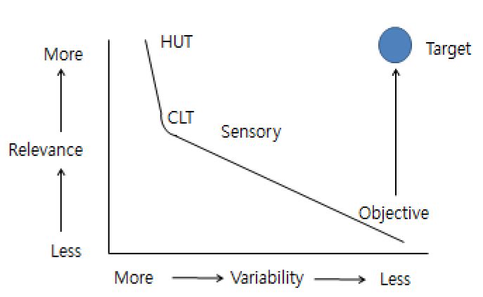
Among the subjective test methods, a HUT should be most relevant since it is conducted by users for their actual in-use situation with minimal controlled environments (constraints). However, it produces the most variability in the collected data. In general, there is a trade-off between the relevance and the variability. As the degree of the constraints (or restriction) increases, its variability would be reduced, but become less relevant in representing the real world.
Meanwhile, objective test methods have been used since they have distinctive advantages over the subjective tests as shown in Table 1. They may not be, however, well correlated with the subjective evaluation results. It should not be surprising to observe that their results are contradictory. For example, product-A which has the higher mechanical strength than product-B may be evaluated weaker by a person, and vice versa.
In short, we have a challenging issue in developing an objective test method, i.e., how to improve relevance while maintaining its reproducibility.
Fig. 1 shows that the target of an objective evaluation method should have the relevance of the HUT while maintaining its reproducibility.
2.1 Subjective data acquisition methods
For a subjective test method, three ways of acquiring data are available:
1) Percentage (%) of the Preference in a Poll
This method is commonly used when two products are compared. In this method, testers are requested to select a product between Product-A and Product- B based on their preference. A percentage of the preference (or poll) is assigned to each product. If more than two products are available, then a round-robin test would be required.
2) Rank Order
This method is used to rank many products. The testers are requested to rank the products from top-to-bottom. A numerical value from 1 to 10 (for 10 products) may be assigned to each product.
3) Rating
It is used to rate a product with a numerical number. Two scaling methods may be employed here.
i) Monadic scale
In this method, a tester is requested to evaluate only one product at a time. The tester is to assign a numerical value within the given range, for example, from 1 for Poor to 5 for Excellent.2)
ii) Magnitude estimate
In contrast with the monadic scale where a range of assigned value is limited, in this method a tester can provide a rating value without any limit. This method has a tendency to allow much broader range in values than the monadic scale. For example, each panelist may be required to mark each product along intensity scale from 1 for Poor to 99 for Excellent. 3)
Table 2 compares the advantages and disadvantages of these methods.
Table 2.
Comparison of subjective data acquisition methods
It should be noted, however, that none of these data acquisition methods should provide linear-scale numbers. For example, in a paired-comparison test, both persons may prefer Product-A to Product-B. However, an intensity of their preference might be significantly different. One person may prefer Product-A much more than Product-B while the other may prefer it marginally. Likewise, a person might perceive the gap between rank 1 and 2 differently from that of the difference between 9 and 10, although the difference is 1 for both.
Meanwhile, a physical measurement such as weight, length, temperature, and pressure provides number on a linear scale. For example, an intensity of the difference remains the same. A weight difference between 100 kg and 150 kg is 50 kg and exactly the same as the difference between 50 kg and 100 kg. Likewise, a 10 degree temperature difference between two objects should be the same between 10℃ and 20℃ and that between 90℃ and 100℃.
To develop an objective evaluation method which can replace subjective evaluation method, it is necessary to convert non-linear subjective evaluation numbers into linear- scale values.
Hallmark has developed an objective tissue softness regression model which has a relatively high correlation with the sensory panel’s softness rating data.4) His regression model, however, would be expected to differ if another scaling method were employed. For instance, the tissue softness regression model developed by Beuther, et al., using different rating scale values turns out quite differently from that of Hallmark.5)
2.2 Linear scale (or interval scale) from a paired-comparison test by Thurstone
Table 2 shows that a paired-comparison test has high discriminatory power while being simple to use. Meanwhile, it should be most difficult to analyze the data since only a relative % of the preference is obtained from the test.
Thurstone has developed a theory of “A Law of Comparative Judgment”.6) This theory is to generate linear (or interval) scale values from paired-comparison tests. The theory appears rather complex involving several statistical theories. The outcome is, however, surprisingly simple and straightforward to use. The theory is simply to “convert percentages” of preferences to a linear scale by determining deviations along the normal curve. The deviations are on a linear-scale, and commonly referred to as the Thurstone Interval Scale.6-8)
2.3 The Thurstone interval-scale theory: illustration
To illustrate the Thurstone theory of obtaining interval scale values from paired-comparison tests, we assume that 200 persons have tested a paired-comparison test for 4 products (A, B, C, and D).
This would require a total of 6 paired-comparison tests, i.e., 1) A vs. B, 2) A vs. C, 3) A vs. D, 4) B vs. C, 5) B vs. D, 6) C vs. D. The required number (N) of paired-comparison tests for n products can be determined from N = n(n-1)/2. For n = 4, N = 4 × 3 ÷ 2 = 6.
In a paired-comparison test, a person is requested to select one between two which he prefers. In the original Thurstone theory, selecting ‘No preference’ should be allowed. Frequently, however, the persons may have difficulty making a selection when they do not find any noticeable difference between the two products. In this case, it seems more reasonable to allow them to select ‘No preference’. Later, no preference data may be excluded for analysis or may be divided into half and added to each selection.
Now, let’s assume that among 200 persons we have the following results:
・ Persons with Preference for A: 125
・ Persons with Preference for B: 45
・ Persons with No preference: 30
Then, 30 persons are divided by 2 and added to each preference. This gives:
The following are the steps for converting the paired-comparison preference data into Thurstone interval scale.
Step 1: Construct raw matrix
The raw matrix is a matrix from tabulating the responses of the persons from a paired-comparison test.
Let us assume that Table 3 is the raw data matrix constructed from the round-robin paired-comparison tests for the four products A, B, C, and D by 200 persons.
In the table, each cell is read as a product in the column is preferred to the product in the row. A diagonal line is drawn in the table to indicate the counterpart product. For example, in the table 140 means that 140 persons among 200 persons selected product-A while 60 persons selected product-B.
Step 2: Construct the preference matrix, P from the raw matrix
Preference matrix, P, is constructed by dividing the preference number of each product by the total number of the testers. In the above example, the preference of A is calculated as 0.70 (= 140 ÷ 200 × 100).
Table 3. Raw data matrix from the Round-Robin paired-comparison tests
Table 4 is the preference matrix constructed from Table 3.
Table 3.
Raw data matrix from the Round-Robin paired-comparison tests
The Raw Date Matrix
| A | B | C | D | |
|---|---|---|---|---|
| A | 100 | 60 | 140 | 80 |
| B | 140 | 100 | 188 | 130 |
| C | 60 | 12 | 100 | 20 |
| D | 120 | 70 | 180 | 100 |
Table 4.
The preference matrix constructed from the raw data matrix
| A | B | C | D | |
|---|---|---|---|---|
| A | 0.50 | 0.30 | 0.70 | 0.40 |
| B | 0.70 | 0.50 | 0.94 | 0.65 |
| C | 0.30 | 0.06 | 0.50 | 0.10 |
| D | 0.60 | 0.35 | 0.90 | 0.50 |
Step 3: Construct the Z-Matrix from the P-Matrix This is the most critical step.
Here Z is called “normal deviate” and it may be obtained from: 1) normal deviate vs. % preference curve,7) 2) tail area of unit normal distribution8), and 3) statistic software such as SAS.9)
According to the Thurstone theory, Z-value should be on linear scale (or interval scale). Thus, the Thurstone interval scale theory is about obtaining Z (normal deviate) value from P (% of preference).
Table 5 shows various Z-values and their corresponding P-values to illustrate how to construct a normal deviate (Z) vs. % of Preference (P) from the tail-area of unit-normal distribution.8) Z-values change from 0.0 to 1.0 by tenth at left column, and change from 0.00 to 0.09 at top row by hundredth. When Z-value is 0.2 at left column and 0.05 at top row, Z-value becomes 0.2 + 0.05 = 0.25. When Z-value is 0.25, % of Preference (P) is 0.401, which is roughly 0.40.
Table 5.
Tail area of unit normal distribution
| Z | 0.00 | ..... | 0.05 | ..... | 0.09 |
|---|---|---|---|---|---|
| 0.0 ..... | 0.500 | ..... | 0.480 | ..... | 0.461 |
| 0.2 ..... | ..... | ..... | 0.401 | ..... | ..... |
| 0.5 ..... | 0.309 | ..... | ..... | ..... | ..... |
| 1.0 ..... | 0.159 | ..... | ..... | ..... | ..... |
Note that from the table, Z should be positive when P > 0.5. For example, when P = 0.5 (i.e., A:B = 50:5), then Z = 0.0. When P ≒ 0.40 (i.e., A:B = 40:60), then the Z-value of B becomes 0.25 whereas Z-value of A becomes 0.
From the table, a curve of normal deviate vs. % of the preference (P) may be constructed, as shown in Fig. 2.7)
Fig. 2 shows a curve of normal deviate vs. % of preference (P).7) It shows several important characteristics
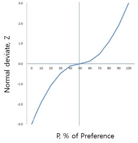
First, the shape of the curve is symmetrical at the point (P = 50% and Z = 0). This simply means that a Z value of P greater than 50% corresponds to Z value (negative) of 100 – P. So, Z value of P = 40% should have the same absolute value as P = 60%. This would be expected from the raw data matrix in Table 3.
Second, Z-values increase non-linearly, but monotonically. This explains why the interval scale values should be directionally consistent with subevaluation numbers such as P (%-preference), rank order, or rating number. Being the shape of the curve is not linear, however, P values should not be treated as interval (i.e., linear) scale. This means it would be meaningless to develop a regression model based on %-preference data.
Third, Fig. 2 shows that Z-value increases rapidly at a high P of around 70% or greater, or decreases rapidly at a low P of around 30%. Around these values, a small change in P would result in a large change in Z-value. This would be very undesirable for obtaining reliable and reproducible results. To avoid this pitfall, it would be cautioned not to test a pair of products when their preferences are expected widely different, say at least by 40% (i.e., 70% - 30%).
As a quick reference, Table 6 shows % Preference vs. Z-value (Interval scale value). In the table, for example, it would be expected to win almost 70% when its Z-value is 0.50. Thus, Z-value should be used as an indicator to predict %-preference in a paired-comparison test.
Meanwhile, we assume Table 7 is the Z-matrix constructed from the P-matrix in Table 4.
Table 6.
%-Preference vs . Z-value (interval scale value)
| % Preference | Z-value (Interval scale value) |
|---|---|
| 50/50 | 0 |
| 60/40 | 0.25 |
| 69/31 | 0.50 |
| 86/14 | 1.0 |
| 93/7 | 1.5 |
| 98/2 | 2.0 |
Table 7.
The Z-Matrix from the preference matrix, P
| A | B | C | D | |
|---|---|---|---|---|
| A | 0 | -0.47 | 2.33 | -0.12 |
| B | 0.47 | 0 | 0.25 | 0.52 |
| C | -2.33 | -0.25 | 0 | 1.04 |
| D | 0.12 | -0.52 | -1.04 | 0 |
Step 4: Get the average Z-values from the Z-matrix and finalize the interval scale values
This step is to get the average Z-value of each product from the Z-matrix and finalize their interval scale values.
It should be more convenient to deal with all positive Z-values. The finalization is to make all Z-values positive. This can be easily done by making the largest negative z-value zero.
Table 8 shows the results. In the table, 0.44 is added to each value to make Product A’s interval scale zero. The table is read by taking the product in each column as preferred to the product in each row. For example, Product A is preferred to Product B by a Z-value of 0.47, while Product B is less preferred to A by a Z-value of -0.47.
The last row in the table indicates the final Z-values of the four products. These form the interval scale which can be treated the same as a linear scale such as that of temperature, length, and weight.
It is remarkable that the interval scale values can be obtained from the simplest, round-robin paired-comparison test. It is expected that the consumer products industry in particular will find benefit from the application of this method, because converting subjective evaluations into objective data is desirable.
3. Subgrouping method
3.1 Critical issues with the Thurstone theory for paired-comparison tests
So far, it has demonstrated to obtain the Thurstone interval scale from a round-robin paired-comparison test for 4 products. For the test, 6 paired-comparison tests were required. There are two critical issues with obtain the Thurstone interval scale from a paired-comparison test
First, the required number of paired-comparison tests would increase dramatically as the number of products being tested (n) increases. For example, if you have 10 products for comparison tests, a total number of required tests would be N= 10*9/2 = 45! It may not be practical to conduct paired-comparison tests when a number of products is too large.
Secondly, as shown in Figure 2, Thurstone scaling values are extremely sensitive to a change in %-Preference when P value is high, i.e., greater than 70%, corresponding to Z-value of approximately 0.5. So, it is advisable that a pair whose Z-value is larger than 0.5 should not be put in a paired-comparison test if one wishes to obtain reliable, reproducible data.
3.2 A partial Round-Robin paired-comparison tests for subgroups
These two critical issues should be solved simultaneously by a judicious experiment design for paired- comparison tests. Specifically, this should be achieved by dividing the whole group into several subgroups. Then, a partial round-robin paired-comparison test should be performed for each subgroup. It is critical that one product should be included in two adjacent subgroups.
To illustrate this concept, we assume that we have 10 products for paired-comparison tests. This would require a total of 45 paired-comparison tests. To begin, we rank them approximately andclassify them into three subgroups in a hierarchical order, as shown in Table 9. In the table, shouldbe noted that one product should be in adjacent groups as a reference (or anchored) product. For example, D appears in both Groups I and II, and G in Groups II and III.
Table 9 suggests that if A were paired with B, it would be preferred to B by 95:5 as estimated from Table 6. Such pairing, however, would not be desirable and should be avoided since Z-value is extremely sensitive to a small change in the preference matrix as discussed earlier.
In following these steps, it would require only 18 paired-comparison tests whereas the full round-robin tests would require 45 paired-comparison tests, resulting in a reduction of 60%!
Now, let us assume that Table 10 is the Z-matrix constructed from a round-robin test in Table 9. In the table, two products, D and G are used as the anchored products. In the table, notice that the sum of the interval scale values in each group becomes 0. The original interval scale data indicates that the reference products, D and G, should have different Z-values.
Table 9.
Subgrouping for Round-Robin comparison tests
| Group I | A | No. of tests = 4 × 3/2 = 6 |
|---|---|---|
| B | ||
| C | ||
| D | ||
| Group II | D | No. of tests = 4 × 3/2 = 6 |
| E | ||
| F | ||
| G | ||
| Group III | G | No. of tests = 4 × 3/2 = 6 |
| H | ||
| I | ||
| J | ||
| N = 18 (vs. 45 for the conventional) | ||
Table 10.
Initial and final interval scale values for Table 9
| Original | Final | ||
|---|---|---|---|
| Group I | A | 0.24 | 1.59 |
| B | 0.16 | 1.51 | |
| C | -0.12 | 1.24 | |
| D | -0.28 | 1.08 | |
| Group II | D | 0.35 | 1.08 |
| E | 0.0 | 0.73 | |
| F | -0.05 | 0.68 | |
| G | -0.30 | 0.43 | |
| Group III | G | 0.25 | 0.43 |
| H | 0.05 | 0.23 | |
| I | -0.12 | 0.06 | |
| J | -0.18 | 0 |
Since the Thurstone interval scale is linear, wecan treat them as ordinary numbers. In the table, Product-J in Group III has the lowest value. We may set this value to zero by adding 0.18 to each row in every group. The final result is shown in the last column of Table 10. It now shows that the anchored products, D and G, have identical values, respectively.
Thus, it is demonstrated that the critical issues with conducting many products for round-robin comparison tests should be resolved by classifying the total group into several subgroups.
4. Conclusions
Availability of relevant and reliable subjective evaluation data is necessary for developing an objective test method which can replaces a subjective test method.
A main problem with subjective evaluation data including a paired-comparison test data is that it is not on a linear-scale. Thurstone has developed a theory of “the Law of Comparative Judgment” which allows one to convert the %-preference in a paired-comparison to a linear (or an interval-scale). Once %-preference is converted to an interval scale, it can be treated as objective numbers.
When more than two products are to be compared with each other, a round-robin test for each pairs would be required. The number of required paired-comparison tests(N) would increase dramatically as the number of product (n) for testing would increase, according to N = n (n-1)/2.
It would be impractical to conduct a full round-robin test if n is too large. This problem should be solved by classifying the total group into several small groups, consisting of 3 - 4 products per subgroup. By doing so, it not only cane reduce N, but can also obtain more reliable, reproducible data.
Converting paired-comparison data to a Thurstone interval scale should make it possible to develop objective test methods which should be able to replace subjective tests. Furthermore, it can be used to develop an empirical (or regression) model which can predict an outcome of a paired-comparison test.
